Optimal Transport I

Problem 1066: In a 2D grid representing a campus, there are n people and m bikes (n <= m). The location of each person and bike is represented by 2D coordinates on the grid. We want to minimize the sum of distances between all possible assignments of people to bikes, where the distance between a person and a bike is calculated using the Manhattan distance.

One approach is to use dynamic programming: sequentially assign each person to a bike, considering the minimum sum of distances achievable with the current bike assignment. The bike assignment status can be represented by a bitmask of length m: 1 indicates the bike has been assigned, and 0 indicates it has not. Therefore, there are a total of 2^m possible assignment states. Since we consider each person sequentially, the complexity of this algorithm is n*2^m. While this is an inefficient algorithm, the constraints on n and m in the original problem are very small: n <= m <= 10, making this approach acceptable. Alternatively, if we view people and bikes as probability distributions on a plane, we can use the optimal transport algorithm to solve this problem.

Optimal transport, initially proposed by the French mathematician Monge for constructing defensive fortifications for the military, has been extensively applied in recent years in various fields, including machine learning. For instance, it can be used to compute the similarity between two data distributions and to train Generative Adversarial Networks (GANs).

In our problem, if we treat people and bikes as two discrete uniform probability distributions, the cost we seek to minimize is that of optimal transport. However, an additional condition is required: n = m, as optimal transport generally assumes balanced probability distributions. In our case, this means the total number of bikes must equal the total number of people. We can use the open-source POT package to solve the optimal transport problem.

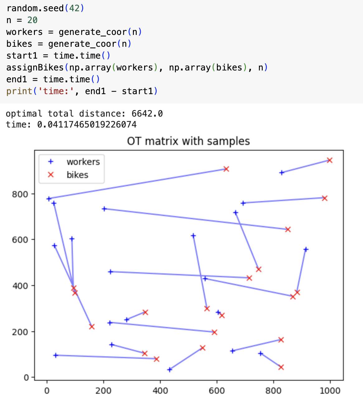
Let a and b represent the probability distributions of people and bikes, respectively. Since each person is assigned only one bike and vice versa (under the condition n = m), a = b = (1/n,...,1/n). Additionally, we know the cost between people and bikes (represented by C) is the Manhattan distance. Therefore, we can write a function to compute the result of optimal transport (where "cityblock" in C represents the Manhattan distance) and visualize the specific transport method.

import ot
import ot.plot


def assignBikes(workers, bikes, n):
   a, b = np.ones((n,)) / n, np.ones((n,)) / n
   C = ot.dist(workers, bikes, 'cityblock')


   G0 = ot.emd(a, b, C)
   dist = ot.emd2(a, b, C) * n
   print('optimal total distance:', dist)


   pl.figure(1)
   ot.plot.plot2D_samples_mat(workers, bikes, G0, c=[.5, .5, 1])
   pl.plot(workers[:, 0], workers[:, 1], '+b', label='workers')
   pl.plot(bikes[:, 0], bikes[:, 1], 'xr', label='bikes')
   pl.legend(loc=0)
   pl.title('OT matrix with samples')

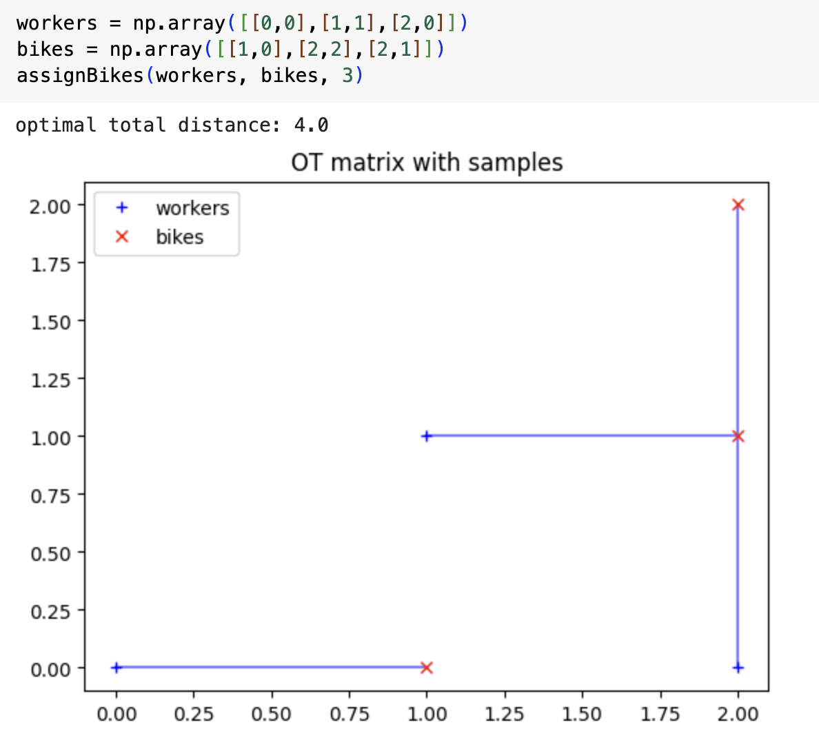
A simple example:

It's worth noting that the complexity of the optimal transport algorithm is only O(n^3 log(n)), which is much more efficient than the dynamic programming algorithm with a complexity of O(n 2^n).

In a more complex example (n = 20) below, the optimal transport algorithm takes 0.04 seconds, while dynamic programming requires 12.9 seconds.

back